By Alan Zhang, Mandy Lee, Yikai (Mike) Mao

1. Introduction
2. Methodology
   1. Data Collection
      1. Raw Data
   2. Model Building
      1. Hidden Markov Model (HMM)
      2. Long Short-Term Memory (LSTM)
3. Conclusion
4. Mentors

Introduction

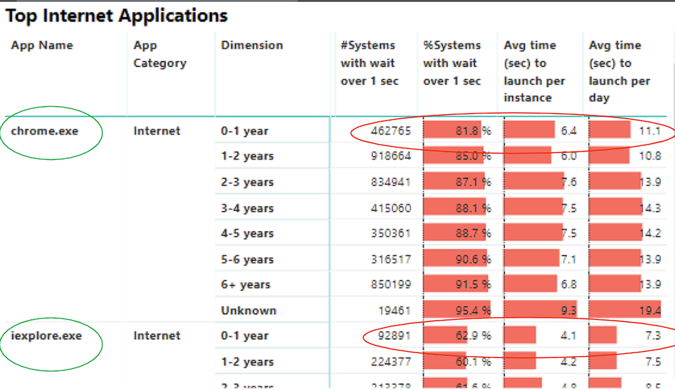
According to a research conducted by Intel, a 0-1 year old computer takes an average of 11 seconds to launch Google Chrome. Our hypothesis is that this data is gathered from across the globe and the minimum PC specification is much lower in markets outside of the U.S. This increased wait time creates a subpar computing experience and hampers productivity. Fortunately, we believe that data science can help. Our proposed solution involves launching applications before the user needs them, which can eliminate the waiting time. To achieve this, we developed software that that collects usage data when the user logs on. This data is then processed and stored in a database. We used eight weeks of data we have collected, we trained two models: a Hidden Markov Model and a Long-Short Term Memory Model. These models are ideal for modeling sequential data and help us understand how a user interacts with their machine. The Hidden Markov Model predicts the sequence of applications used, while the LSTM model identifies which application is a potential candidate for pre-launching based on its predicted hourly usage. More information about our implementation details can be found below.

Methodology

Data Collection

We used Intel’s X Library Software Development Kit (XLSDK) to develop a system usage data collector on our Windows 10 device. Upon signing into the system, the collector automatically launches and begins tracking all foreground applications. To ensure its reliability in real-world scenarios, we followed these principles:

1. Robustness and Resilience

   To ensure that our program continues to run without requiring human intervention in the event of errors during deployment, we have implemented defensive coding practices. We have verified the data type and range of variables before feeding them into functions. If an error occurs, we log the error type, the file that generated the error, the line number within the file, and the timestamp. This enables us to identify faulty code while reviewing error logs. Through this approach and rigorous testing, we were able to keep our collector running without errors for eight weeks.

2. Privacy Compliance

   To obtain the name of the foreground window application, we must locate the application’s file path, which may contain Personal Identifiable Information (PII) such as a person’s full legal name. To prevent the collection of PII, we have implemented a process to remove any PII from the file path before storing the collected information. For example, if a user has named their system after their legal name, we exclude the full file path to prevent the collection of PII.

3. Efficiency

   We have optimized the code to reduce the impact on system resources, such as CPU and memory usage, by minimizing unnecessary processing and data transfer. This is crucial as we want the application to run continuously in the background while the computer is on. To achieve this, we only allocate the minimum necessary memory to arrays and expand them as needed, ensuring efficient use of system resources.

4. Compatibility

   We have designed the data collector to be compatible with a wide range of languages by changing our collected strings from ANSI to UNICODE to capture foreign characters. This enables us to accurately capture and store data in different languages, ensuring compatibility with various software applications and operating systems.

Raw Data

Here is a snippet of the 8 week of raw data

MEASUREMENT_TIME	ID_INPUT	VALUE	PRIVATE_DATA
2023-02-22 15:16:11.231	3	Discord.exe	0
2023-02-22 15:16:22.683	3	explorer.exe	0
2023-02-22 15:16:31.341	3	firefox.exe	0
2023-02-22 15:17:01.379	3	Teams.exe	0
2023-02-22 15:17:03.605	3	firefox.exe	0
2023-02-22 15:17:34.905	3	explorer.exe	0
2023-02-22 15:17:37.986	3	Code.exe	0
2023-02-22 15:17:56.994	3	firefox.exe	0
2023-02-22 15:17:58.600	3	Code.exe	0
2023-02-22 15:18:01.654	3	firefox.exe	0
2023-02-22 15:18:16.922	3	CodeSetup.tmp	0
2023-02-22 15:18:20.113	3	firefox.exe	0
2023-02-22 15:22:00.113	3	explorer.exe	0
2023-02-22 15:22:03.071	3	Code.exe	0
2023-02-22 15:24:27.911	3	firefox.exe	0

If you want to learn about the obstacles we faced, click here:

1. Unfamiliar Environment

As the programming language C was not initially included in our Data Science curriculum, we had to quickly learn and adapt to this new coding environment within a tight 2-week deadline. One of the initial challenges we encountered was the lack of immediate feedback on our code. Unlike in Python Jupyter Notebooks, where we could easily run a block of code and print out results to diagnose any issues, in Visual Studio, we had to rely on our judgment that the entire code block was functioning correctly. Fortunately, when we asked our mentor for guidance, they were able to teach us how to use the debugging mode, which significantly improved our ability to identify and fix errors in our code.

2. Oudated Documentation/Setting up the Environment

Everybody dreads setting up the coding environment for a new role. It's the least enjoyable part of the coding experience. For us, we had to install internal software using documentation that was written 6 years ago. Some of the changes that happened since then are not documented and not well tested. For regular software, we can just use an installer and open the application. This, however, requires us to follow specific instructions such as where to extract the folder and how to edit the configuration files. This was particularly frustrating because the engineers implemented a fix to the program without throughout testing and documentation. Our mentors were unable to help because they already had the environment set up and are not familiar with the propagated changes. This caused us a precious week to read through the document code to trace the error and get started on writing the code.

3. Win32 API

The official API documentation is helpful but lacks examples, making it challenging to use. When we tried to get the title of the foreground window the user is currently on, we located two functions: GetWindowTextA, and GetWindowTextW. Since GetWindowTextA is the first result on Google, I used that function until I discovered that it is not capturing the text of a window that has Chinese characters. Upon further investigation, we discovered that A stands for ANSI and return an ANSI string and W stands for wide-character which returns a Unicode string. It would not be easy to spot such a mistake at first glance because the API description for these two functions is almost identical. The only difference is that the output variable is named LPWSTR for the GetWindowTextW function and LPSTR for the GetWindowTextA function. These information are not readily available on forums such as StackExchange, making this task a lot harder.

Model Building

To gain insights into how users interact with their computers, we utilized the Hidden Markov Model and Long-Short Term Memory model to identify patterns from the data. The Hidden Markov Model is based on Bayes’ Theorem and can predict the next application a user will use based on their previous application. Assuming conditional independence, we can employ Naive Bayes’ Theorem to map out the sequence of applications that a user is likely to use on a given day.

Hidden Markov Model (HMM)

Hidden Markov Model is commonly used to model sequential data, which makes this a particularly good choice to predict the next application that the user will open. To understand HMM, we must understand Bayes’ Rule.

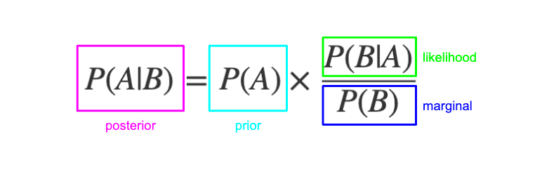
In simple terms, this means that the likelihood of event A happening after event B has occurred is the probability of both events A and B happening together, divided by the probability of event B happening on its own. In our scenario, we just need to tally up the number of times an application (e.g., Zoom) is used after Google Chrome has been used. This can help us generate a list of applications that are commonly used following the use of a specific application. Below are the application that are most likely to follow our ten most used application overall.

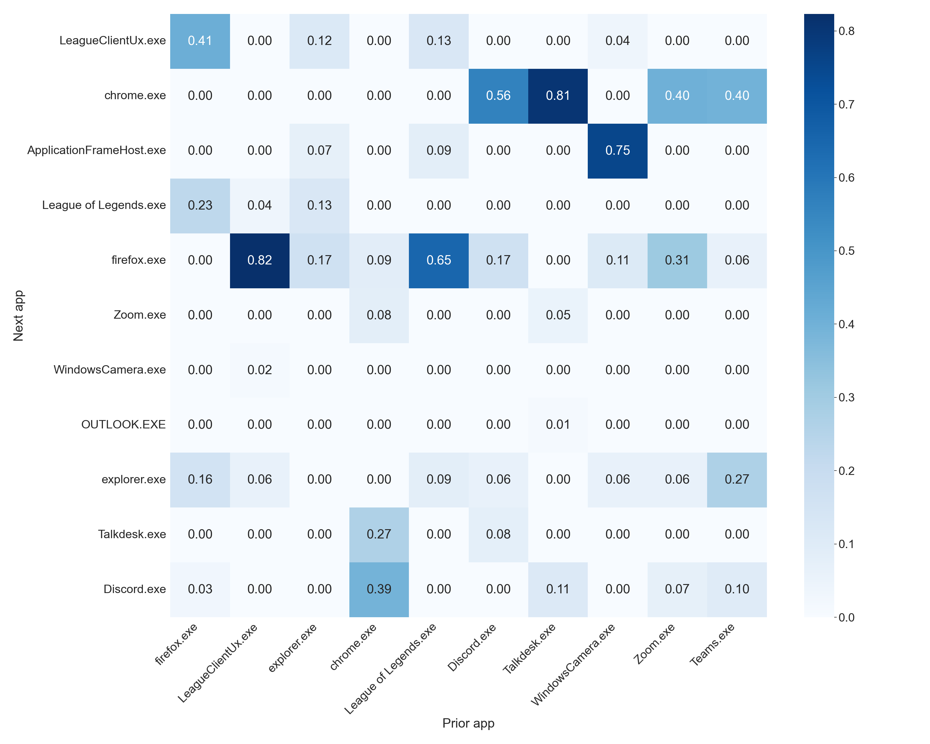
Overall, the model seems to be picking up some trends such as the tendency to switch to Google Chrome after using Discord, Talkdesk, Zoom, and Microsoft Teams, which aligns with my work-related tasks as these applications are commonly used in my work environment. It is also identified that when I have League of Legends open, I will most likely switch over to Firefox, which is consistent with my leisure activities.

Anecdotally, the model appears to be accurately capturing my usage patterns. Now, lets evaluate evaluate the model’s performance using statistics and metrics. We chose accuracy as it is the most appropriate statistic for a classifiaction task. To measure accuracy, we assessed whether the predicted application falls within the top N, where N is a number, applications predicted based on the previous software used. We allow for an acceptable margin of error, so the model’s predictions are not penalized too harshly. This helps ensure that the model produces useful recommendations.

Top N	Accuracy
1	48%
2	65%
3	75%

To model a user’s sequence of applications on a given day, we can apply naive Bayes’ theorem and chain the predictions to continue predicting the next application until we reach a stop token. For this approach to work, we must assume that the events are independent from each other. This means that the probability of the next application is only predicted based on the previous application and not on the sequence of applications that precede it. To determine the final sequence of applications used, we find the sequence of applications that has the highest product of the conditional probabilities in a process called maximum likelihood estimation.

Long Short-Term Memory (LSTM)

Now that we have a sequence of applications, it is important to determine which of these applications is significant. We will measure importance using two metrics: predicted hourly usage and frequency of usage. To forecast hourly application usage, we narrowed our focus to the web browser Firefox and built an initial LSTM model. We selected Firefox because users typically spend a significant portion of their computer time browsing the web, whether for reading news, watching videos, or communicating with colleagues. By training our model to recognize usage patterns for one web browser, we can scale it to learn patterns across different applications.

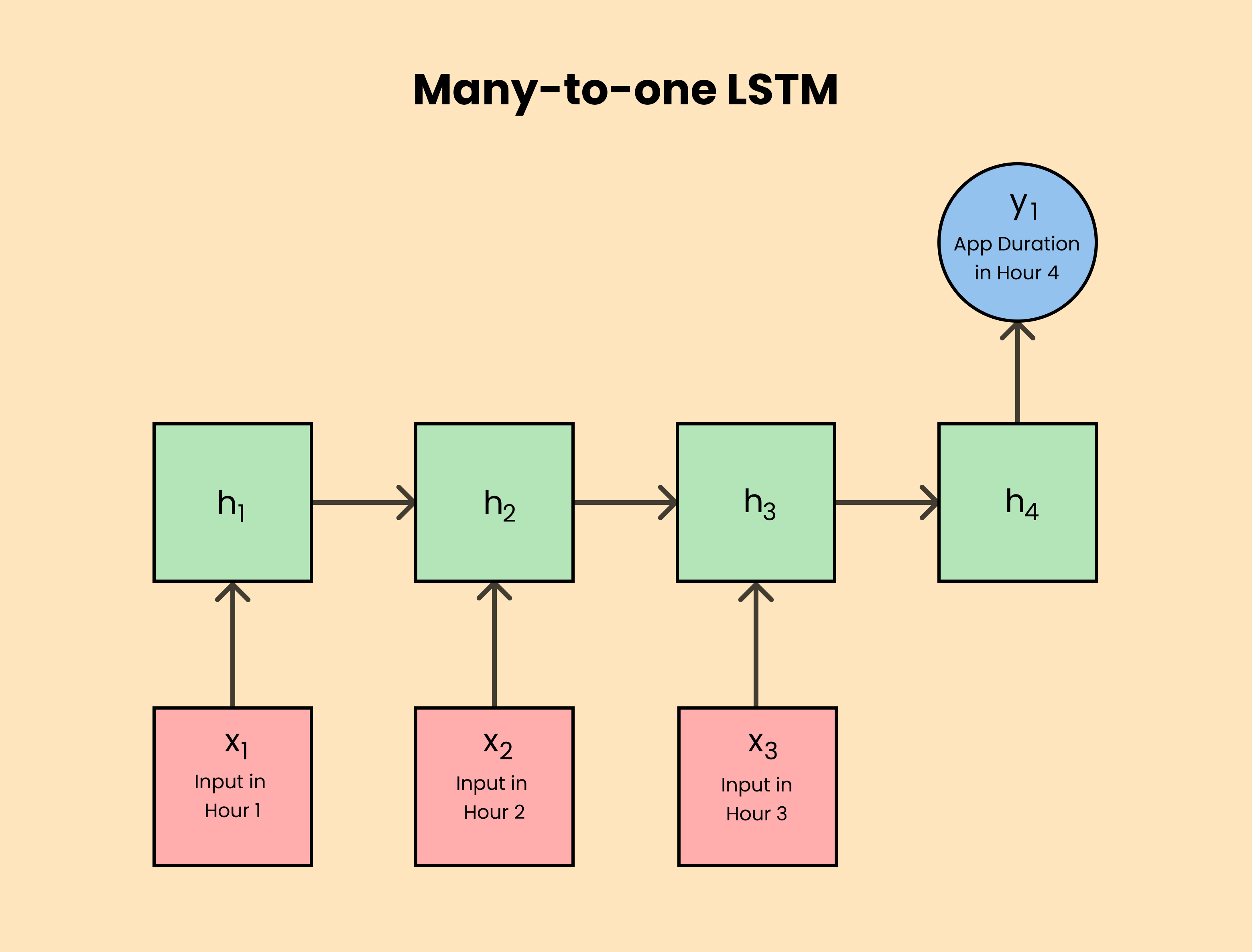
We have decided to use Tensorflow’s Keras package, a high-level neural network API for Python, to implement LSTMs as a layer in a neural network. In an LSTM network, the hidden state is updated at each time step by combining the values of the input, forget, and output gates, and the memory cells are updated accordingly. This process allows the LSTM to selectively store or forget information over a long period of time, making it well-suited for tasks such as speech recognition, natural language processing, and time-series prediction. Just like the figure below, data such as process names and dates are imported and multiple hidden layers are updated to output the next name/duration of the processes.

Input Data:

• Numerical feature:
  • Scaled app duration
• Binary features:
  • Is_Weekend - 1 represents a weekend and -1 a week day
  • Is_Winter_Holiday - 1 represents a winter holiday and -1 for every other date.
• One-hot-encoded features:
  • Minute of the Hour - a $1\times60$ vector
  • Hour of the Day - a $1\times24$ vector
  • Day of the Week - a $1\times7$ vector
  • Day of the Month - a $1\times31$ vector
  • Day of the Year - a $1\times366$ vector
  • Month of the Year - a $1\times12$ vector

Explanation of our Input Selection:

We chose those one-hot-encoded features in order to study usage pattern at an hourly level and the time the application is opened can be used to find patterns in how long it was open for given the similiar conditions. In addtion, is_weekend, and is_winter_holiday are selected to distinguish between the holiday season and school season since the data collection process started in mid-December and ended in February. These variables separate the data into categories so that the computer can distinguish usage pattern for a productive day from an entertainment day. We also think information in the previous hour period might be a useful indicator for the prediction in the next hour so we included a Min-Max scaled duration as another feature.

Performance Metric:

Our model uses Mean Squared Error as the loss function for training. For a regression problem, MSE allows the model to update its parameters through back-propagation due to its differentiability. In addition, we included another human-interpretable measurement, accuracy, to better understand our model’s performance. This accuracy is based on whether the prediction and the target are within an arbitrary margin of error (we chose three thresholds, 5, 10, and 60 seconds). This is to give the model a bit of leeway for when it predicts the amplitude correctly but is off by a few seconds to a minute.

Results:

Metric	Train Result	Test Result
MSE Loss	0.0038	0.1384
Accuracy within 5s	84%	79%
Accuracy within 10s	85%	80%
Accuracy within 10s	86%	82%

When we compare the graph of the model’s performance to the table of results, we can see that the model does not perform well on the testing set. The graph shows that the model fails to capture most of the spikes, which is in contrast to the high test accuracy reported in the table. This discrepancy may be due to the fact that the model is correctly predicting many 0s, which suggests that the accuracy metric may not be a good evaluation tool.

To address this issue, we could adjust our evaluation metric to penalize incorrect amplitude predictions more severely while reducing rewards for correctly predicting 0s. This approach aims to address the class imbalance between active and inactive usage and encourage the model to focus on learning the amplitude of usage time more accurately.

Moreover, the graph suggests that the model is able to effectively learn from the training set, but struggles to forecast future patterns. We hypothesize that the poor performance on unseen data is due to the insufficient dataset, as there are features in the testing set, such as day of the year and month, which are not present in the training set and thus make the model difficult to generalize.

Conclusion

We have developed software and models that serve as fundamental building blocks for constructing more complex and accurate models to identify suitable applications for pre-launch. By developing our own collector, we have gained insights into responsible data collection and good practices for acquiring and storing data. Our collector is memory-efficient and can run 24/7 without human intervention. If you wish to collect your own data and run it against our model, you can clone our GitHub repository and add the script to your Task Scheduler. Detailed instructions are available in the repository.

Although our HMM model does not achieve the highest accuracy, it indicates that the model is generalizing well rather than simply memorizing and overfitting to the training data. Our LSTM model requires further work, and we suggest exploring modifications such as changing the metrics to one more suitable for this regression task, as the current accuracy measurement can be misleading. Moreover, the high accuracy of the model mostly results from correctly predicting zeros rather than timing and amplitude values. We can alter our test set to include only amplitudes or rebalance the amplitude and zero points to more effectively evaluate the model on an unseen dataset. Last but not least, we hope to collect additional data for the dataset to capture more consistent usage patterns.

We encourage those interested in the project to build upon what we have developed by following our GitHub repository. All instructions are available in the README.md file.

Mentors

We would like to express our gratitude to all the mentors at the Intel DCA & Telemetry team who provided invaluable guidance and support throughout this project. None of this would be possible without them. Special thanks to Jamel for his passion and mentorship, teaching us not only how to be better data scientists but also well-rounded engineers. Bijan for creating an environment that encourages us to step out of our comfort zones and continuously learn. Sruti for sharing her expertise and teaching us how to create our own HMM model. Oumaima for providing endless suggestions on how to improve our model by experimenting with different inputs. Praveen for teaching us how to automate our data collection process. Lastly, we would like to thank Teresa for her dedication and ensuring that we received timely feedback from the mentors. Their guidance has been instrumental in our growth and development as data scientists.

• Bijan Arbab
• Jamel Tayeb
• Sruti Sahani
• Oumaima Makhlouk
• Teresa Rexin
• Praveen Polasam
• Chansik Im